
Studio notes
The Deceptive Backtest: Why a Trading Bot That Wins on History Loses in Live Markets
On pure random data, the best of 174 strategies backtested well, then went flat. Spot overfitting, look-ahead and survivorship bias, and test with walk-forward.
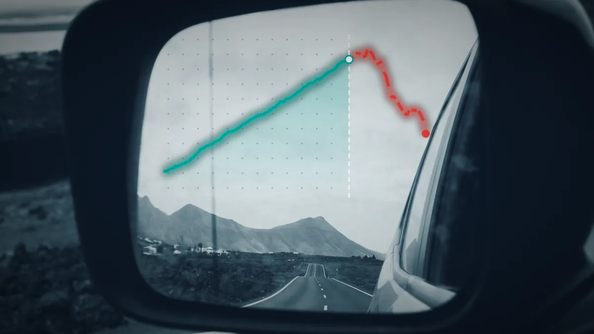
I ran a simple experiment. I generated ten years of fake daily prices that were completely random. There is no pattern in that data, so no strategy can have a real edge on it. Then I tested 174 variants of a classic moving-average crossover on the first five years and kept the best one. I repeated the whole thing on 200 different random series.
On average, the "best" variant had an annualised Sharpe ratio of 0.68 over the first five years. Show that equity curve to someone and it looks like a respectable strategy. Over the next five years, the same variant averaged a Sharpe of exactly 0.00, and it lost money in 48% of runs.
This article is for traders and developers who build or buy trading bots. It walks through the ways a backtest lies to you: overfitting, data snooping, look-ahead bias, survivorship bias, and costs that never made it into the simulation. Then it shows how walk-forward testing and genuinely out-of-sample data help you catch each one. None of these methods guarantees a profit. They only make it harder to fool yourself.
The experiment: the best strategy on meaningless data
The rule was simple: go long when the short moving average is above the long one, go short when it is below. The short window ranged from 5 to 50 days and the long window from 20 to 200 days. A signal built from each day's close was executed from the next day. Results across 200 runs:
| Scenario | Mean Sharpe of best variant, years 1–5 | Sharpe of the same variant, years 6–10 | Share of runs losing money in years 6–10 |
|---|---|---|---|
| No costs | 0.68 | 0.00 | 48% |
| 0.1% cost per position change | 0.61 | -0.08 | 56% |
| With a look-ahead bug | 1.07 | 0.76 | 6% |
The first row is pure overfitting. The strategy learned nothing about the market; we simply found the variant that happened to fit the noise of those five years. The second row shows how costs turn zero into a loss. The third row is the most dangerous, and we will come back to it: one small bug made even the out-of-sample test look "profitable" on completely random data.
We ran this code with Python 3.13 and NumPy 2.5 on synthetic data, and the numbers above are its output. It is a teaching tool, not a trading bot, and it has not been tested on real market data or a live account.
import numpy as np

def sharpe(r):
    return np.sqrt(252) * r.mean() / r.std() if r.std() > 0 else 0.0

def ma(x, n):
    c = np.cumsum(np.insert(x, 0, 0.0))
    out = np.full(len(x), np.nan)
    out[n-1:] = (c[n:] - c[:-n]) / n
    return out

def run(seed, cost=0.0):
    ret = np.random.default_rng(seed).normal(0.0, 0.01, 2520)  # pure noise: no real edge
    price = 100 * np.cumprod(1 + ret)
    half, results = 1260, []
    for fast in range(5, 55, 5):
        for slow in range(20, 210, 10):
            if slow <= fast:
                continue
            pos = np.nan_to_num(np.sign(ma(price, fast) - ma(price, slow)))
            pos = np.roll(pos, 1); pos[0] = 0                   # trade on the next bar
            pnl = pos * ret - cost * np.abs(np.diff(pos, prepend=0))
            results.append((sharpe(pnl[:half]), sharpe(pnl[half:])))
    results = np.array(results)
    best = results[:, 0].argmax()
    return results[best]          # (in-sample Sharpe, out-of-sample Sharpe)
Overfitting: when the bot memorises noise
Overfitting means tuning a rule so closely to past data that it memorises that period's random accidents instead of anything the market repeats. Every parameter, filter or exception you add is another degree of freedom. With enough of them, you can draw any equity curve you like.
Every trial is a lottery ticket
David Bailey, Marcos López de Prado and their co-authors put numbers on this in "Pseudo-Mathematics and Financial Charlatanism" (Notices of the AMS, 2014). With only five years of data, you should try no more than about 45 independent configurations. With 45 trials, the best one is expected to show an in-sample Sharpe of 1 even if every one of them has a true Sharpe of zero. With two years of data, that happens after just seven trials.
I checked this with a simulation. Each time, I built N independent strategies with no edge on five years of daily data and recorded the highest Sharpe:
| Independent trials | Mean highest Sharpe (simulation) | Bailey & López de Prado formula |
|---|---|---|
| 10 | 0.70 | 0.70 |
| 45 | 1.00 | 1.00 |
| 100 | 1.12 | 1.13 |
| 1,000 | 1.45 | 1.46 |
A five-year Sharpe of 1.45 looks excellent to most people. Here it is just the best of a thousand coin-tossing runs.
There was a subtle point in the first experiment too. The 174 moving-average variants are similar to one another, not independent. Their best Sharpe (0.68) was about the size you would expect from the best of ten independent trials. What matters is the number of genuinely different ideas, not the number of rows in your optimisation grid. That does not make broad searches safe; it just makes the risk harder to count.
Evidence from the real world
This is not only theory. Two field studies:
- 888 algorithms on Quantopian. Wiecki and colleagues (Journal of Investing, 2016) studied algorithms with at least six months of true out-of-sample performance. The backtest Sharpe ratio had almost no power to predict later Sharpe (R² below 0.025). And the more backtests an author had run on a strategy, the wider the gap between backtest and later performance.
- 215 strategies from investment banks. Suhonen, Lennkh and Perez (Journal of Portfolio Management, 2017) reported a median 73% drop in Sharpe ratio from backtest to live trading. For the most complex strategies, the drop was more than 30 percentage points larger than for the simplest ones.
The practical lesson: complexity has a price. If a simpler rule gives roughly the same result, keep the simpler one.
Data snooping: count the whole path
Data snooping means testing so many ideas on one dataset that one of them eventually looks good by luck. Those ideas are not only parameters. Every time you look at the chart and think "it should skip Fridays", you have run a test, even if you never wrote the code.
Academic research takes this seriously. Harvey, Liu and Zhu (Review of Financial Studies, 2016), looking at the hundreds of factors tested on the same data, argued that a new factor should clear a t-statistic above 3, not the usual 2. Back in 2000, Halbert White introduced the Reality Check in Econometrica, a test that judges the best rule while accounting for the fact that it was picked from many rules that were tried.
The Deflated Sharpe Ratio
A more practical tool for bot builders is Bailey and López de Prado's Deflated Sharpe Ratio (Journal of Portfolio Management, 2014). It accounts for how many trials you ran, how long your data is, and how far returns are from a normal distribution (skew and fat tails). Its output is a probability: the chance that the true Sharpe exceeds the best Sharpe you would expect from that many trials with no edge.
Here is a worked example I calculated: a strategy with an annualised Sharpe of 1.5 over three years of daily data, skew of -0.5 and kurtosis of 5. I assumed the trials are independent and that the spread of their Sharpe ratios comes from noise alone:
| Best of how many trials? | Sharpe expected from luck alone | Probability it is real (DSR) |
|---|---|---|
| 1 | 0 | 0.99 |
| 10 | 0.91 | 0.84 |
| 100 | 1.46 | 0.53 |
The same 1.5 is convincing if it was your only idea. If it was the best of a hundred, it is close to a coin flip. That is why a research log is your best defence: record every idea, every variant and every failure, so you know your real N.
Bailey and colleagues also proposed the Probability of Backtest Overfitting (PBO). The data is cut into blocks; each time, some blocks are used to pick the best configuration and the rest to evaluate it. If the in-sample winner often lands below the median out of sample, your selection process is overfitting, not just one strategy.
Look-ahead bias: the bug out-of-sample testing will not catch
Look again at the third row of the first table. In that version, the signal was built from today's close and traded on today's return. In other words, the bot knew a price that did not yet exist when it made the decision. The result: a Sharpe of 0.76 in years six to ten on completely random data, with 94% of runs profitable out of sample.
This is the key point. Splitting your data protects you from overfitting, but not from bugs. If the code peeks at the future, it peeks in the test data too. The only place this bug gets exposed is a live account.
Common sources of look-ahead in trading bots:
- Making a decision mid-bar using that bar's close, or entering at the very close that produced the signal.
- Indicators that rewrite their past values later (repainting), such as some zigzag and fractal indicators.
- Normalising or scaling with the mean and standard deviation of the whole dataset.
- Fundamental or economic data stamped with the period it describes rather than the date it was released.
- Bar timestamp mistakes: does the timestamp mark the bar's open or its close? Is the server time zone the same as the data's?
The truncation test: simple and effective
One simple automated test catches most of these. Compute the signal once on the full data and once on data cut off right after time t. The signal value at t must be identical in both cases. If removing the future changes it, the code is using the future.
import numpy as np
import pandas as pd

def check_no_lookahead(signal_fn, prices: pd.Series, checkpoints=(300, 600, 900)):
    full = signal_fn(prices)
    for t in checkpoints:
        partial = signal_fn(prices.iloc[: t + 1])
        if not np.isclose(full.iloc[t], partial.iloc[t], equal_nan=True):
            return False, t
    return True, None
We ran this function on three sample signals. A signal using ordinary moving averages passed. A centred moving average (center=True in pandas) and a z-score normalised with the whole series' mean both failed at the first checkpoint. The test will not catch every leak; a wrong release date, for example, can only be found by checking the data itself. But it belongs in your bot's CI and should run every time the signal logic changes.
There is a companion check: delay execution by one bar. An edge that disappears completely with a one-bar delay either depends heavily on execution speed or came from the future. Either way, it needs a closer look.
Survivorship bias: data that erased the losers
Say you take today's top 50 cryptocurrencies, or the current members of a stock index, and test your strategy on their last ten years. The problem is that these are the winners of those ten years. Symbols that crashed, were delisted or were dropped by the exchange are not in your data. Without knowing it, your backtest only traded survivors.
Elton, Gruber and Blake (Review of Financial Studies, 1996) measured this effect in mutual funds. Funds that disappear from the data usually disappear because they performed poorly, so averaging only the survivors makes the picture look better than reality.
What to do:
- Build the tradable universe point in time: on each day, include only the symbols that were tradable that day.
- Get data for delisted symbols too. If your data provider does not have it, state that limitation in your backtest report.
- For single-symbol strategies, ask why that symbol was chosen. If the answer is "because it did well in the past", that is survivorship bias too.
Costs, slippage and execution
In the first experiment, a cost of just 0.1% per position change pushed the mean out-of-sample Sharpe from zero to -0.08, and that strategy traded rarely. The higher your turnover, the bigger the share costs take.
The minimum every backtest should include:
- The real spread during the hours your bot actually trades, not the average or minimum spread.
- Commission and, where relevant, swap or funding rates for overnight positions or perpetual contracts.
- Slippage, especially around news and for market orders.
- A conservative assumption for limit orders: price touching your level does not mean your order was filled.
A simple test: double the costs. If the strategy dies at double costs, its safety margin is too thin to rely on. We cover execution issues such as dropped connections and rejected orders in more depth in our article "Why trading bots fail live" on this site.
Walk-forward and out-of-sample testing, done right
Splitting your data is the only serious defence against overfitting, provided you do it properly.
What walk-forward shows
In walk-forward testing, you optimise parameters on one time window, trade the next window you have not seen, roll forward and repeat. At the end, you stitch together only the out-of-sample pieces and evaluate those.
I ran this on the same random data: optimise on two years, trade the following six months, repeat across ten years. The best variant in each optimisation window averaged a Sharpe of 1.05. The stitched out-of-sample curve had a Sharpe of -0.02. Walk-forward reported exactly what was true: there is no edge here.
Rules for not fooling yourself
- Lock away the last part of your data. For example, set aside the final 20% on day one and run your final strategy on it only once, at the very end. If you go back and change anything after seeing that result, it is no longer out-of-sample.
- Window lengths are parameters too. If you tried ten walk-forward window lengths and reported the best, you have overfitted again, just one level higher.
- Look for plateaus, not peaks. Choose parameters whose neighbours give similar results. If a 23-day window is great but 21 and 25 lose money, you have found noise.
- Purging and embargo. If each label or trade outcome spans several days, say "the five-day forward return", training samples whose spans overlap the test period leak information. In Advances in Financial Machine Learning, López de Prado recommends removing those samples and leaving a short gap after each test period. For machine-learning bots this step is essential; ordinary shuffled k-fold cross-validation is misleading on financial time series.
- Cover different market regimes. Your test period should include trends and choppy ranges, calm periods and crises. A short, quiet out-of-sample period proves very little.
After all that, the final step before a live account is a parallel run on a demo account or with very small size. The goal of this stage is not profit; it is a trade-by-trade comparison between the live bot and a backtest of the same days. Differences in entry prices, trade counts and timing are early signs of a look-ahead leak or a wrong cost model.
Checklist before you switch the bot on
- How many ideas and variants did you actually try? Is that number in your report?
- Given that many trials and that much data, is the Deflated Sharpe Ratio still convincing?
- Does a truncation test for look-ahead run in CI? Does the result still hold with a one-bar delay?
- Is the universe on each date exactly what existed on that date, delisted symbols included?
- Are real costs, spread, slippage and swap modelled? Does the strategy survive double costs?
- Did the result come from walk-forward, with parameters on a plateau rather than a peak?
- Has the locked final holdout been opened only once?
- If labels overlap, were purging and embargo applied?
- Does the test period cover several different market regimes?
- Has a demo or small-size parallel run been compared with a backtest of the same days?
If the answer to any of these is "no" or "I don't know", the backtest Sharpe has not proven anything yet.
Conclusion
A backtest is a tool for rejecting bad ideas, not for proving good ones. On completely random data, 45 trials produced a Sharpe of 1 and a thousand trials produced 1.45. A one-line bug produced a "profitable" out-of-sample result. So the backtest number alone is never enough. You need to know how many times you tried, that the code does not peek at the future, that the data includes the losers, that costs are realistic, and that the result came from walk-forward testing.
If your bot hands trading decisions to an AI model, our article "AI Agent Trading Bots: The Model Sends the Order, but You Own It" covers the controls you need to build outside the model.
This article is educational and is not investment advice or a promise of profit. No testing method guarantees future returns. If you would like us to review your backtesting process, historical data or bot signal code with you, get in touch through the Order page on the Behvandi website.
Comments
No comments yet. Be the first to write one.